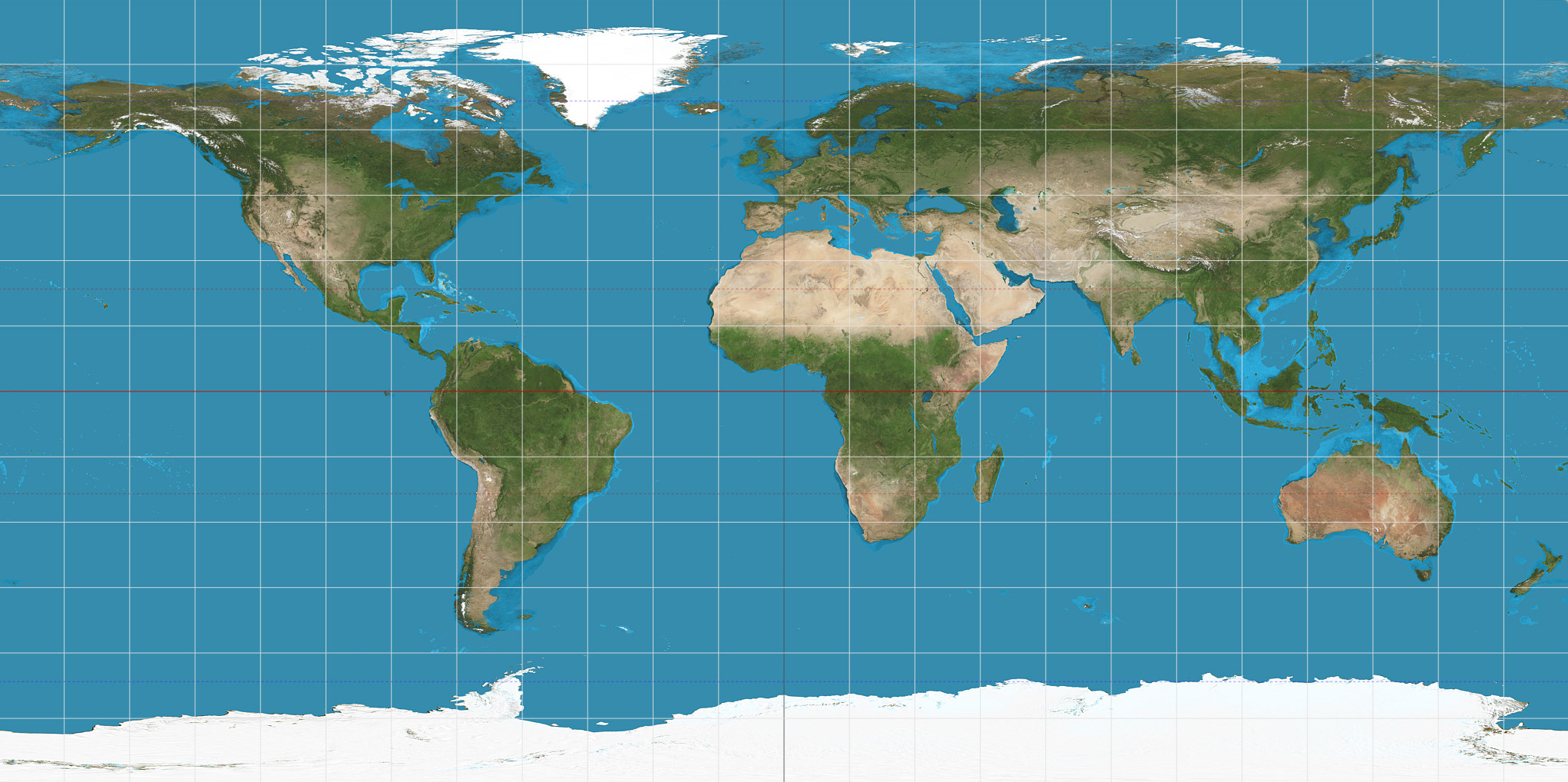
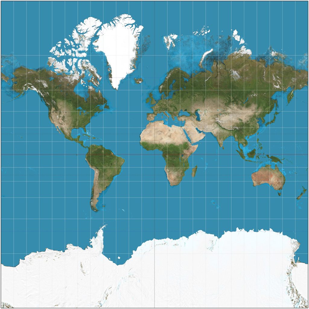
It’s well known that the Mercator projection makes a certain kind of navigation easy: Follow a compass at a constant bearing, and the map shows you where you’ll end up. The problem with the Mercator projection is that the north and south poles end up grossly exaggerated.
I want to solve this problem with a map projection that’s worse in every other measurable way.
I want a projection that follows a loxodrome:
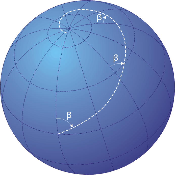
Loxodromes, also called rhumb lines, are curves on a sphere that intersect each meridian at a constant angle. The equation for this is:
L(t) = 2 tan-1(ebt)
Where L is the latitude, t is the longitude, and b = tan(
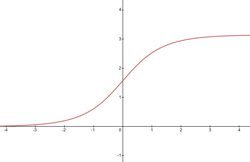
This curve asymptotically approaches 0 and π as it heads off towards either infinity. This is because the loxodrome spirals endlessly around the poles. As tempting as it is to have a projection that stretches off to both infinities, it would be nice to be able to hang it in on my wall.
The motivation for what’s about to happen next came to me from the thought “What if we just squished the x-axis down so L(t) appeared to be a straight line?” Instead of scaling down the x-axis, we can also scale the input to L with another function, g(x). Since we want L(g(x)) creates a straight line, that means the derivative of L'(g(x)) is a constant. So let’s get the derivative of L(g(x)):
L'(g(x)) = b *g'(x) * sech(b * g(x))
Where sech() is the hyperbolic secant.
Since this derivative is a constant, we can turn it into a differential equation of the form:
b *g'(x) * sech(b * g(x)) = 1
Solving this equation for g(t) gives us:
g(x) = sinh-1(tan(bk + x))/b
Where k is a constant, and sinh is the hyperbolic sine function. We’ll see what k does in a bit. First let’s plug this g into L(t) to see what we get with q = 1.
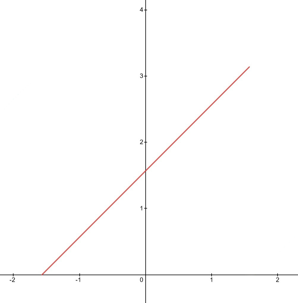
Great! We have a line that goes from (-π/2, 0) to (π/2, π) Would be nice to have it go from (0, 0) to (π, π) though. And oh, hey, that’s where k comes in. If we set k to π/2b then we’ll get:
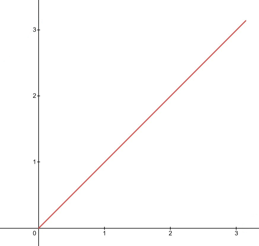
There we go. This leaves our equation as:
g(x) = sinh-1(tan(π/2 + x))/b
Let’s review what we now have. We started with L(t), which maps longitudes to the latitude of a loxodrome. We then found a function g(x) that scales x such that L(g(x)) is a straight line. So g(x) is a function that maps an x-coordinate to a longitude, and L(g(x)) maps x-coordinates to longitudes. We also have a constant b defined by the angle the loxodrome intersects each meridian at.
This is great for mapping points along the loxodrome to the 2d plane, but to make a proper projection we need to map every point on the sphere to the 2d plane. So we need a 2d function that maps spherical coordinates to the 2d plane. We already have a parameterized equation for the spherical coordinates of the loxodrome from way back above:
S(x) = {L(x), x}
So we can add a 2nd parameter to this equation that will give us every point on the sphere:
S(x, u) = {L(x), x + u}
Where u is within [-π, π]. With u, we rotate each point on the loxodrome around its latitude so we can sample the entire sphere. Since we’re substituting x with g(t), we can use this equation:
S(t, u) = {L(g(t)), g(t) + u}
Since we know L(g(t)) is a line, we can simplify this to:
S(t, u) = {t, g(t) + u}
And we can express g(t) + u in terms of g(t + v(t, u)), which will be useful in just a second:
v(t, u) = π – t – cot-1(sinh(u – sinh-1(cot(t))))
S(t, u) = {t, g(t+ v(t, u))}
So the spherical coordinate maps to the Cartesian plane through the equations:
x = t+v(t, u)
y = t
Going from the Cartesian plane to the spherical coordinates then:
t = y
u = sinh-1(cot(π – x)) + sinh-1(cot(y))
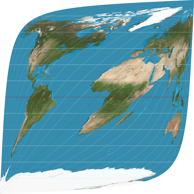
This is why we made v(t, u) earlier. Now that we have a way to determine the inputs to S(t, u) we can finally make our map. Here it is with B = 0:

This is the projection that follows the prime meridian from pole to pole. The reason for the shape is that this is what you get when you limit u to [-π, π). If we ignore this bound we’ll see that the map repeats features. If we had infinite pixels to zoom into, we’d see that the map features would actually repeat infinitely as you approach the edge of the map.

If you want to see other angles, I made this little tool you can mess around with. Notice that at a loxodrome angle of -45 degrees, something interesting happens. I’ll leave it as an exercise to the reader to understand why.
Earth’s rotation:
Loxodrome Angle: